traductor

martes, 27 de abril de 2021

Los salvavidas de la ciencia


Los salvavidas de la ciencia

El apellido Bosch se reconoce fácilmente como vinculado al mundo de la ingeniería y la industria, debido sobre todo Robert Bosch, inventor de la bujía y fundador de la compañía que lleva su nombre. Su sobrino Carl no se quedó atrás y fue también un poderoso industrial. Pero además se le considera uno de los dos científicos cuyos hallazgos han servido para salvar más vidas: 2.720 millones, según la web ScienceHeroes.com. Estos son los descubrimientos científicos, y sus protagonistas, a los que debemos un homenaje como grandes salvavidas de la ciencia.

1. Fertilizantes

Fritz Haber y Carl Bosch

El nitrógeno es un nutriente esencial para las plantas, pero no pueden tomarlo directamente en la forma gaseosa inerte presente en la atmósfera; necesitan que los microbios hagan el trabajo por ellas. Hasta comienzos del siglo XX sólo el estiércol y el nitrato de Chile, procedente del guano de las aves, podían suministrar el nitrógeno a las plantas de forma aprovechable.

Carl Bosch y Fritz Haber. Crédito: BASF y Nobel Foundation

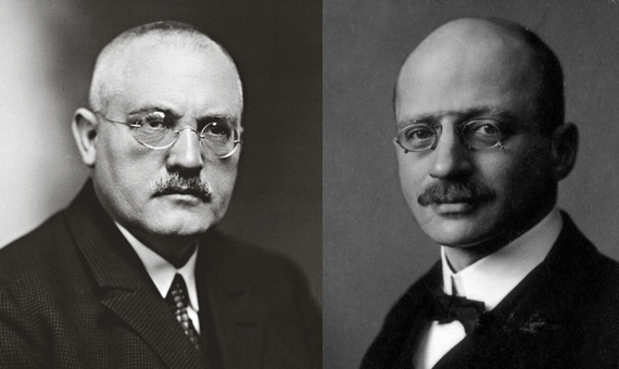
Esto era así hasta que el 3 de julio de 1909 el químico alemán Fritz Haber (9 de diciembre de 1868- 29 de enero de 1934) logró por primera vez unir nitrógeno e hidrógeno, a alta presión y temperatura y mediante el uso de un catalizador metálico, para producir amoníaco. En la compañía BASF, Carl Bosch (27 de agosto de 1874 –  26 de abril de 1940) se encargó de transformar el experimento de Haber en un proceso a escala industrial. Ambos recibirían el premio Nobel de Química, Haber en 1918 y Bosch en 1931.

El proceso de Haber-Bosch cambió el mundo: se calcula que la alimentación de la mitad de la población mundial depende de los fertilizantes derivados de él. Pero tiene un reverso oscuro; este método permitió la fabricación a gran escala de los explosivos modernos, responsables de entre 100 y 150 millones de muertes en el último siglo. Con ocasión de la Primera Guerra Mundial, Haber fue además un entusiasta impulsor de las armas químicas, creando el gas cloro cuyo uso en las trincheras supervisaba él mismo. Se cree que esta actividad de Haber provocó el suicidio de su primera esposa, la también química Clara Immerwahr, de convicciones pacifistas.

2. Grupos sanguíneos y transfusiones

Karl Landsteiner y Richard Lewisohn

Con 1.094 millones de vidas salvadas, los artífices del descubrimiento de los grupos sanguíneos y de las técnicas de transfusión merecen el segundo puesto en el podio de los científicos salvadores. La lista de aportaciones a este campo de la ciencia es inmensa, dado que las primeras transfusiones se intentaron ya poco después de que en 1628 el médico inglés William Harvey (1 de abril de 1578 – 3 de junio de 1657) hiciera la primera descripción detallada y completa de la circulación sanguínea.

Karl Landsteiner en su laboratorio, en 1901. Autor: desconocido

Entre los siglos XVII y XIX proliferaron los intentos de transfundir sangre entre animales, entre humanos, o entre ambos, a menudo con consecuencias fatales. Con el nacimiento del siglo XX, el austríaco Karl Landsteiner (14 de junio de 1868- 26 de junio de 1943) comprendió que la aglutinación de sangre de diferentes personas se debía a la existencia de distintos grupos sanguíneos, que nombró A, B y C. Por su parte y mientras trataba de vincular las enfermedades mentales con las de la sangre, en 1907 el psiquiatra checo Jan Janský definió los cuatro grupos que hoy conocemos como el sistema AB0. En 1937 Landsteiner, en colaboración con Alexander S. Wiener, añadió el descubrimiento del factor Rhesus o Rh, pero ya antes las transfusiones sanguíneas habían empezado a tomar forma científica.

Las primeras transfusiones empleando criterios de compatibilidad se realizaron en el Hospital Monte Sinaí de Nueva York a cargo de Reuben Ottenberg, que identificó la existencia de un grupo donante universal. Pero fue el cirujano germano-estadounidense Richard Lewisohn (12 de julio de 1875 – 11 de agosto de 1961), del mismo hospital, quien en 1915 aplicó con éxito el anticoagulante citrato sódico para conservar las muestras refrigeradas durante dos o tres semanas, lo que abrió la posibilidad de almacenar la sangre en bancos. El hallazgo llegó justo a tiempo, ya que las transfusiones salvarían miles de vidas durante la Primera Guerra Mundial.

3. Microbios y sepsis

Louis Pasteur y Joseph Lister

Hasta el siglo XIX todavía se creía que los seres vivos podían surgir espontáneamente de la nada; por ejemplo y según Aristóteles, los pulgones nacían de las gotas de rocío. La existencia de los microbios había comenzado a postularse desde mediados del siglo XVI, pero no fue hasta los experimentos de fermentación del químico francés Louis Pasteur (27 de diciembre de 1822 – 28 de septiembre de 1895) cuando pudo confirmarse que la generación espontánea no existía, y que todo ser vivo nacía de otro ser vivo.

Louis Pasteur realizando un experimento. Autor: desconocido

Pasteur descubrió que los microorganismos eran responsables de la contaminación de las bebidas, y que esto no sucedía cuando se esterilizaban por calor y después se mantenían en recipientes cerrados. En 1865 Pasteur patentó su método, que hoy conocemos como pasteurización. Pero además de sus aplicaciones industriales, el químico intuyó que los microbios eran responsables de las enfermedades a través de las infecciones.

Las ideas de Pasteur llegaron al conocimiento del cirujano británico Joseph Lister (5 de abril de 1827 – 10 de febrero de 1912). Por entonces, las infecciones de las heridas se atribuían a las miasmas, o aire podrido. Pero cuando Lister supo que el trabajo de Pasteur demostraba la contaminación de los alimentos incluso en ausencia de aire, decidió aplicar una esterilización química al material y a las heridas en sus operaciones. Para ello empleó ácido carbólico, hoy llamado fenol. La web ScienceHeroes.com no llega a estimar el número de vidas salvadas por los hallazgos de Pasteur y Lister, pero es evidente lo que todos les debemos a ambos, incluso en lo más cotidiano: en 1879 un químico de Missuri creó un antiséptico bucal al que llamó Listerine.

4. Vacunas

Edward Jenner

El del médico y cirujano inglés Edward Jenner (17 de mayo de 1749 – 27 de enero de 1823) es un caso de constancia y método, pero también de una audacia que hoy le habría llevado a prisión. Contrariamente a lo que a veces se presenta, la idea de la vacunación no le surgió de un momento “eureka”: en su época se practicaba la variolización, o inoculación de costras o pus de la viruela en personas sanas para protegerlas de lo que entonces era una terrible plaga.

Retrato de Edward Jenner. Autor: James Northcote

En ocasiones funcionaba, pero en otros casos los resultados eran fatales. Varios médicos antes que Jenner habían notado que los ganaderos contraían una versión benigna, la viruela vacuna, permaneciendo inmunes a la enfermedad humana, e incluso habían ensayado inoculaciones con este material. El de Jenner fue el primer estudio extenso sobre la materia, para el que eligió como primer paciente a un niño de ocho años, James Phipps, hijo de su jardinero.

Por fortuna, el método funcionó: la vacunación, o inoculación con la viruela vacuna, protegió al niño de la posterior exposición a material de la enfermedad humana. Sin embargo, los experimentos de Jenner inicialmente suscitaron escepticismo e incluso burlas. Desde sus ensayos iniciales en 1796, tuvieron que transcurrir 44 años, con Jenner ya fallecido, para que el gobierno británico adoptara oficialmente la vacunación.

En 1979 y como fruto de una extensa campaña, la Organización Mundial de la Salud declaró la erradicación de la viruela. El trabajo de Jenner ha salvado unos 530 millones de vidas, pero a ellas deberíamos añadir las muertes evitadas por otras vacunas contra numerosas enfermedades mortales. Estas vacunas tienen sus propios héroes, pero todas ellas se derivan del trabajo pionero de Jenner.

5. Cloración del agua

Linn Enslow y Abel Wolman

La falta de acceso a agua potable continúa siendo hoy una de las principales causas de mortalidad en los países en desarrollo. Según la Organización Mundial de la Salud, 1,6 millones de personas mueren cada año por enfermedades diarreicas vinculadas al agua contaminada; el 90% son niños menores de cinco años. Pero hasta bien entrado el siglo XX, el agua era un factor de riesgo sanitario en todo el mundo: los países más industrializados ya contaban con canalizaciones para el abastecimiento, pero a menudo la calidad era deficiente, y el grifo podía servir de entrada a infecciones letales como el cólera, el tifus o la disentería.

Abel Wolman. Crédito: Johns Hopkins University

A finales del siglo XIX comenzó a experimentarse con la cloración del agua como método de esterilización, pero a veces el remedio era peor que la enfermedad, dado que el cloro es tóxico. Encontrar el punto exacto para aprovechar sus propiedades antisépticas sin envenenar a la población parecía un reto demasiado espinoso, hasta que un ingeniero sanitario del Departamento de Salud Pública del estado de Maryland (EEUU) llamado Abel Wolman (10 de junio de 1892 – 22 de febrero de 1989) se propuso dar con la fórmula precisa. Para ello contó con la ayuda del químico Linn Enslow (26 de febrero de 1891 – 3 de noviembre de 1957) . Entre ambos diseñaron en 1919 un método estandarizado para clorar el agua de la red de Baltimore.

Aunque inicialmente las autoridades eran reacias a verter cloro en sus canalizaciones de agua, el sistema de Wolman y Enslow se probó fiable y seguro, extendiéndose por todo el mundo en unas décadas. La cloración del agua ha sido calificada como uno de los mayores avances en salud pública del pasado milenio, que según la web ScienceHeroes.com ha salvado 177 millones de vidas en todo el mundo.

Javier Yanes 

@yanes68


viernes, 23 de abril de 2021

Neutrobots, nanotecnología para tratar tumores celebrales


Neutrobots, nanotecnología para tratar tumores celebrales 

Un híbrido entre células, componentes de bacterias y nanorobots consigue atravesar la barrera hematoencefálica para administrar fármacos y tratar tumores cerebrales en ratones. 

Angiografía del cerebro. Técnica que permite observar los vasos sanguíneos no visibles mediante radiología convencional

En los últimos años y en lo que al tratamiento de enfermedades cerebrales o neurológicas se refiere, los científicos se han topado, y nunca mejor dicho, con una barrera difícil de franquear a la hora de desarrollar nuevos tratamientos para tratar una amplia variedad de enfermedades que van desde el Parkinson o el Alzheimer, hasta llegar a los propios tumores cerebrales. Hablamos de la barrera hematoencefálica, una fina capa de células que rodea a los vasos sanguíneos del cerebro y que no por fina cumple con menor eficacia su función, la de evitar el flujo de sustancias indeseadas entre el sistema circulatorio y nuestro encéfalo.

Hoy la barrera hematoencefálica es objeto de numerosos estudios. Así por ejemplo, la semana pasada informábamos como una investigación centrada en las diferencias entre las barreras hematoencefálicas de hombres y mujeres, abría la puerta para sentar las bases sobre como distintas enfermedades neurológicas afectan de manera diferente a los seres humanos según su sexo.

Y es que atravesar esta barrera se ha convertido en la clave para tratar las múltiples afecciones del cerebro, así como para incrementar su efectividad, ya que al ser la mayoría de los fármacos para el tratamiento de enfermedades neurológicas administrados por vía oral o intravenosa, la función protectora de la barrera hematoencefálica motiva que los diferentes tratamientos no alcancen su diana, en este caso el cerebro humano, y cumplan con su propósito.

En este sentido, el de superar esta barrera, a principios de enero también informábamos de como científicos del hospital de Brigham y el Hospital infantil de Boston habían logrado mediante nanotecnología de polímeros atravesar la misma para administrar diferentes moléculas que podrían tener un efecto beneficioso y terapéutico.

Thank you for watching

Neutrobot, el nuevo avance de la nanotecnología

Ahora, en un paso más allá, un equipo de investigadores dirigidos por la doctora Hongyue Zhang, del Instituto de Tecnología de Harbin, en China, han conseguido integrar diferentes componentes de células y bacterias en un microrobot magnético capaz de atravesar la barrera hematoencefálica de ratones sin ser atacados por el sistema inmunológico. Bautizados como "neutrobots" estos consiguieron administrar un tratamiento eficaz para los tumores cerebrales de los ratones estudiados y aumentar la supervivencia de los animales.

Acción de los neutrobots en un tumor cerebral

Acción de los neutrobots en un tumor cerebral

Foto: Zhang et al.

Para construir sus microrobots, los investigadores expusieron neutrófilos de ratón -un tipo de leucocito abundante en la sangre- a partículas de nanogel magnético recubiertas con trozos de membrana de Escherchia coli.Al reconocer a las bacterias como seres extraños, los neutrófilos envolvieron las partículas, transformándose en neutrobots. "Así, los microrobots biohíbridos combinan las capacidades de propulsión y unión de gel magnético con la biocompatibilidad natural y las capacidades de penetración de la barrera hematoencefálica de los neutrófilos, lo que supone una promesa considerable para la administración clínica de fármacos al cerebro" explica Zhang.

Los científicos pusieron a prueba su experimento en un modelo de tumor de ratón. Los neutrobots, cargados con el medicamento contra el cáncer llamado paclitaxel, "pasaron de contrabando" al fármaco a través de la barrera hematoencefálica, liberando después los nanogeles y medicamentos cerca de los tumores cerebrales, lo que se tradujo en una mayor supervivencia de los ratones tratados. Como siguiente paso, Zhang tendrá que desarrollar un sistema de control magnético más fuerte para activar los microrobots en un espacio de trabajo más grande: quizá, todo el cuerpo humano.

Foto: iStock

 https://www.nationalgeographic.com.es/ciencia/neutrobots-nanotecnologia-para-tratar-tumores-celebrales_16725?utm_source=facebook&utm_medium=social&utm_campaign=trafico&

fbclid=IwAR24GDm_SX0R2cI0pvmV7mkIM1woy5spcXfkZH085Ekl4NQfZWeU_8AYbxw

 https://notistecnicas.blogspot.com/2021/04/xenobots-ahora-autoorganizados.html?fbclid=IwAR3vjO4_9tCYGkJw4jaDVUJ5oaEBBsOlPZwYzVRe1fNM_FhLY_gQ6IAcYds

lunes, 19 de abril de 2021

Xenobots, ahora autoorganizados


Xenobots, ahora autoorganizados

Con células embrionarias de ranas se hacen pequeños robots, o xenobots, que se mueven libremente, curan sus lesiones y crean sus propios comportamientos de grupo. 

Esther Megbel

Un equipo de científicos, prosiguiendo unas investigaciones que publicaron a principios de 2020, ha criado una especie de pelusas capaces, como diminutos robots, de desplazarse y ejecutar distintos movimientos, formadas por células embrionarias de rana que se han autoorganizado así. Douglas Blackiston y Michael Levin, biólogos de la Universidad Tufts, y sus colaboradores llaman a estas «criaturas» suyas xenobots, como a sus precursoras de hace un año (que no se autoorganizaban, sino que eran «esculpidas» por los investigadores en conjuntos  de progenitoras de células epidérmicas y cardiacas siguiendo las recomendaciones de un algoritmo). El nombre deriva del nombre científico de la rana de la que se toman las células, Xenopus laevis (la rana de uñas africana). Describen el trabajo en Science Robotics.

Las células de esta nueva versión de los xenobots son células epiteliales de embriones de esas ranas. Las cultivaron durante cuatro días en el laboratorio; ellas mismas se ordenaron de una forma distinta a como lo habrían hecho en el embrión, en concreto como esa especie de bolas de pelusa con movimiento propio. Se mantuvieron activas diez días, pero si se les aportaban nutrientes su existencia se prolongaba bastante.

En esos cuatro días de cultivo desarrollaron medios de desplazamiento: crearon en su superficie unos cilios que, aunque sirven a un propósito distinto en el animal, a los xenobots les valen para moverse por el agua. Los cilios son unas finas protuberancias de la superficie celular, parecidas a pelos, que baten en el medio coordinadamente, de modo que se produce un movimiento coherente y orientado; en los seres humanos, por ejemplo, expulsan gérmenes y partículas de los pulmones, y en las ranas distribuyen homogéneamente el moco sobre su piel. En el experimento, en cambio, propulsan a los xenobots en las húmedas placas de Petri, por superficies no lisas e incluso a través de angostos tubos. Los xenobots, que miden medio milímetro, avanzan a una velocidad de tres centímetros y medio por hora. Cómo se coordinan sus cilios, con patrones espaciales muy concretos, es desconocido.

Los xenobots se comportan casi como un enjambre mientras se propulsan con sus cilios. [Doug Blackiston / Universidad Tufts]. ].

Para poner a prueba la capacidad autocurativa de estos entes, el equipo los lesionaba con pinzas quirúrgicas. Un cuarto de hora después, ya se habían regenerado y ninguno murió prematuramente. Observaron además que se organizaban como un enjambre: limpiaron en media día un entorno cubierto con partículas de óxido de hierro; con sus idas y venidas fueron acumulándolas en pequeños montones.

Levin, Blackiston y sus colaboradores ven este experimento como una primer paso que puede ayudar a la investigación del desarrollo de las agrupaciones celulares. Con los xenobots, por ejemplo, se podría investigar qué estímulo necesitan las células para formar unidades mayores. El equipo querría generar en el futuro robots de material biológico más desarrollados, de uso en biomedicina o como sensores. Los xenobots tienen ya una memoria rudimentaria: los investigadores les incorporaron una proteína fluorescente, gracias a la cual esas pelusas autónomas desprendían una luz verde. Pero cuando se los somete a una fuente de luz azul, su fluorecencia pasa de modo duradero a ser roja. De esa forma, los xenobots guardan en sí un recuerdo de un estímulo con el que entraron en contacto a lo largo de sus recorridos.

Esther Megbel

Referencia: «A cellular platform for the development of synthetic living machines», de Douglas Blackiston et al., en Science Robotics31 de marzo de 2021:
vol. 6, núm. 52, eabf1571.

https://www.investigacionyciencia.es/noticias/xenobots-ahora-autoorganizados-19734?utm_source=boletin&utm_medium=email&utm_campaign=Biolog%C3%ADa+-+Abril+%28II%29


Las incógnitas resueltas desde la publicación del genoma humano, hace 20 años


Las incógnitas resueltas desde la publicación del genoma humano, hace 20 años

La identificación de muchas de las lagunas de la secuencia original ha ofrecido detalles relevantes de la estructura y función de nuestro genoma.

Este año se cumple el vigésimo aniversario de la publicación del primer borrador del genoma humano. [Instituto Nacional de Investigación del Genoma Humano, de los EE.UU.]

La publicación del borrador del genoma humano en 2001 por dos grupos independientes, el Consorcio Internacional para la Secuenciación del Genoma Humano (CISGH) y el equipo de J. Craig Venter, supuso un hito histórico. Por primera vez, se abría la posibilidad de estudiar tramos largos de cada uno de los cromosomas humanos, base por base. Gracias a ello, los investigadores podían empezar a entender cómo estaban ordenados los distintos genes, y cómo se organizaba y estructuraba el ADN circundante que no codificaba proteínas. A pesar de este increíble progreso, el borrador del genoma aún estaba incompleto; faltaban más de 150 millones de bases por identificar. Los avances tecnológicos en los años transcurridos desde entonces han permitido mejorar el borrador, y en 2020 se logró finalmente la secuenciación completa de un cromosoma. Como resultado, están empezando a emerger a la superficie nuevas partes del genoma hasta entonces no descritas, lo que está dando paso a otro emocionante período de descubrimientos biológicos.

¿Qué incluían exactamente los borradores iniciales del genoma? Contenían numerosas regiones intergénicas previamente inexploradas. También incluían la inmensa mayoría de los genes. El CISGH estimó al principio que el genoma contenía entre 30.000 y 40.000 genes codificadores de proteínas, aunque la publicación de un genoma actualizado en 2004, junto con la mejora de las estrategias de predicción de genes, provocó que la cifra se revisara a cerca de 20.000. El genoma de 2004 aportó un mapa de alta resolución de 2850 millones de nucleótidos de la eucromatina. Esta corresponde a las regiones del ADN empaquetadas de una forma más holgada, que están enriquecidas en genes y representan aproximadamente el 92 por ciento del genoma humano.

El genoma de referencia impulsó a la comunidad científica hacia una era de exploración genómica, que redirigió el foco desde los genes individuales hasta estudios más genéricos del genoma completo. Sin embargo, seguía habiendo lagunas en cada uno de los 23 pares de cromosomas humanos, que según las estimaciones contienen más de 150 megabases de secuencias desconocidas. Las mayores lagunas se situaban en regiones enriquecidas con ADN altamente repetitivo o con secuencias para las que existen muchas copias casi idénticas. Al principio, estas secciones fueron difíciles de clonar, secuenciar y ensamblar correctamente. Como resultado, el proyecto del genoma humano infrarrepresentó a propósito tales secuencias repetitivas. Aunque los investigadores tenían una idea muy básica sobre su naturaleza, la organización genómica de alta resolución de la región en cuestión seguía sin concretarse.

El borrador del genoma humano del 2001 abarcó la mayor parte del ADN rico en genes, que se halla empaquetado de forma holgada en el núcleo. Pero seguían existiendo muchas lagunas en regiones muy compactadas y ricas en secuencias repetitivas, que a menudo no se transcriben (en la imagen se exagera la extensión de estas para facilitar la interpretación) (<em>a</em>). Gracias a los avances en secuenciación y bioinformática, hoy es posible estudiar dichas lagunas. Estas incluyen las regiones teloméricas y subteloméricas en los extremos de los cromosomas; las estructuras centroméricas, esenciales para la división celular; y los brazos acrocéntricos, muy cortos y repetitivos. Ahora también pueden analizarse las regiones en las que el ADN está duplicado, ya sea en una única localización o de forma segmentada (<em>b</em>).
El borrador del genoma humano del 2001 abarcó la mayor parte del ADN rico en genes, que se halla empaquetado de forma holgada en el núcleo. Pero seguían existiendo muchas lagunas en regiones muy compactadas y ricas en secuencias repetitivas, que a menudo no se transcriben (en la imagen se exagera la extensión de estas para facilitar la interpretación) (a). Gracias a los avances en secuenciación y bioinformática, hoy es posible estudiar dichas lagunas. Estas incluyen las regiones teloméricas y subteloméricas en los extremos de los cromosomas; las estructuras centroméricas, esenciales para la división celular; y los brazos acrocéntricos, muy cortos y repetitivos. Ahora también pueden analizarse las regiones en las que el ADN está duplicado, ya sea en una única localización o de forma segmentada (b).

En los primeros intentos por identificar las lagunas se empleó la secuenciación de lectura larga para abarcar las secuencias repetitivas, aunque tales lecturas al principio tendían a dar errores. En 2010 aparecieron nuevas oportunidades, gracias a los avances en la capacidad de leer fragmentos más largos de secuencia, junto con el desarrollo de herramientas bioinformáticas escalables. Las lecturas de secuencia de decenas a centenares de kilobases permitieron el estudio de la organización genómica de muchas lagunas de tamaño moderado. Esto permitió conocer algunas de las regiones subteloméricas (ADN muy repetitivo adyacente a las estructuras teloméricas, en los extremos de los cromosomas). También permitió el estudio de la primera secuencia satélite centromérica, en la que se repiten secuencias cortas en tándem durante unas 300 kilobases. De igual forma, se resolvió un subconjunto de duplicaciones segmentadas (secuencias que comparten entre el 90 y 100 por ciento de sus bases y ocupan múltiples localizaciones), muchas de las cuales contenían genes previamente ausentes del genoma de referencia. Sin embargo, muchas de las regiones más grandes ricas en repeticiones, de múltiples megabases de tamaño, seguían siendo inabarcables.  

A lo largo de los últimos años, los datos de lecturas largas muy precisas y de lecturas ultra-largas han resultado esenciales para resolver estas regiones. Han revelado, por vez primera, tramos extremadamente largos de repeticiones en tándem y regiones enriquecidas en duplicaciones segmentadas. Al superar estas barreras técnicas, los científicos están descubriendo ahora extensas regiones ricas en repeticiones que pueden abarcar millones de bases, y constituir así el brazo corto entero de los cromosomas.

Obtener la imagen completa

Sin embargo, los investigadores aún no entienden del todo las razones por las que algunas partes del genoma humano se organizan de la forma en que lo hacen. Alcanzar este conocimiento será, sin lugar a dudas, valioso, porque estas secuencias ricas en repeticiones suelen estar situadas en zonas que son cruciales para la vida. Por ejemplo, los tramos largos de repeticiones de ADN ribosómico (ADNr) codifican componentes de ARN de la maquinaria celular encargada de la síntesis de proteínas y desempeñan un papel importante en la organización nuclear. Y el ADN repetitivo de las estructuras denominadas centrómeros es esencial para una adecuada segregación cromosómica durante la división celular. 

Estas largas tiras de ADN repetitivo vienen con distintos conjuntos de reglas, en términos de su organización y evolución genómicas. También están sujetas a diferente regulación epigenética (modificaciones moleculares en el ADN y en las proteínas asociadas a él que no alteran la secuencia básica del ADN), lo que lleva al ADN repetitivo a diferir de la eucromatina en lo que se refiere a organización, tiempo de replicación y actividad transcripcional. Muchas herramientas y conjuntos de datos del genoma completo todavía no pueden capturar toda esta información de las regiones de ADN extremadamente repetitivas. Por tanto, no se dispone aún de una imagen completa de los factores de transcripción que se unen a ellos, de cómo tales regiones se organizan espacialmente en el núcleo, o de cómo la regulación de estas partes de nuestro genoma cambia durante el desarrollo y en situaciones de enfermedad. En la actualidad, de forma muy parecida a lo que sucedió con la publicación inicial del genoma décadas atrás, los investigadores se enfrentan con un paisaje funcional nuevo e inexplorado del genoma humano. El acceso a esta información impulsará la tecnología y la innovación hacia la inclusión de dichas regiones de repeticiones, ampliando una vez más nuestra comprensión de la biología del genoma.  

El año pasado, se utilizaron secuenciaciones de lecturas muy largas y precisas para reconstruir cromosomas humanos enteros de telómero a telómero. También tuvo lugar la publicación de un genoma de referencia humano casi completo a partir de una línea celular humana «haploide», en la que solo existen cinco lagunas que marcan las zonas de ADNr. En dicha línea, las células tienen dos pares idénticos de cromosomas, lo que simplifica el ensamblaje en comparación con las células humanas típicas (que son diploides, con diferentes cromosomas heredados de la madre y del padre). En conjunto, estos mapas permiten vislumbrar por vez primera, en alta resolución, las regiones centroméricas, las duplicaciones segmentadas, las repeticiones subteloméricas y cada uno de los cinco cromosomas acrocéntricos, que tienen unos brazos muy cortos formados casi exclusivamente por ADN altamente repetitivo en un extremo.

Resulta tentador pensar que los científicos se acercan por fin a la línea de meta. Sin embargo, un único ensamblaje genómico, aunque esté completo con una precisión de secuencia casi perfecta, es una referencia insuficiente a partir de la que poder estudiar la variación en toda la población humana. Los mapas existentes que representan la diversidad a través de las partes eucromáticas del genoma deben extenderse para capturar por completo las regiones repetitivas, en las que el número de copias y la organización de las repeticiones varían entre individuos. Hacerlo requerirá el desarrollo de estrategias para la producción y el análisis rutinarios de genomas humanos diploides completos. El ambicioso objetivo de alcanzar una referencia más completa e integral de la humanidad mejorará, sin duda, nuestra comprensión de la estructura genómica y su papel en las enfermedades humanas, y se alineará con la promesa y el legado del Proyecto del Genoma Humano.

Karen H. Miga/Nature News & Views

Artículo traducido y adaptado por Investigación y Ciencia con permiso de Nature Resarch Group.

La representación más detallada de la célula humana


La representación más detallada de la célula humana hasta la fecha, obtenida por radiografía, resonancia magnética nuclear y microscopia crioelectrónica.


https://russell-kightley.pixels.com/.../animal-cell?fbclid=IwAR3D1fv1r9DNovLTcQu85KVQbBfNdW7uKI_KZuGF4aeO235cVp-eEowpdBw

https://www.instagram.com/ciencias_medicas_biologicas/?fbclid=IwAR3mYYJ2uEvpwqmuu_QNvZ_8TsiwU4YkX8_4_EADqt_fNN0RypfIk0cff4I

viernes, 16 de abril de 2021

La variante D614G del SARS-CoV-2 favorece un estado conformacional abierto

 How did the D614G strain get its increased infectivity?

https://advances.sciencemag.org/content/7/16/eabf3671 @ScienceAdvances

Elegant supercomputer microsecond all-atom simulations suggests open state of the spike protein led to increased receptor binding but easier antibody neutralization (<-good!) via Eric Topol -Elegantes simulaciones de microsegundos en superordenadores sugieren que el estado abierto de la proteína de la espiga conduce a una mayor unión de los receptores pero a una neutralización más fácil de los anticuerpos 

La variante D614G del SARS-CoV-2 favorece un estado conformacional abierto

-The SARS-CoV-2 Spike variant D614G favors an open conformational state- View ORCID ProfileRachael A. Mansbach1,†,‡, View ORCID ProfileSrirupa Chakraborty1,2,†, View ORCID ProfileKien Nguyen1,†, View ORCID ProfileDavid C. Montefiori3, View ORCID ProfileBette Korber1- https://advances.sciencemag.org/content/7/16/eabf3671


The SARS-CoV-2 Spike variant D614G favors an open conformational state

See all authors and affiliations

Science Advances  16 Apr 2021:
Vol. 7, no. 16, eabf3671
DOI: 10.1126/sciadv.abf3671

Abstract

The COVID-19 (coronavirus disease 2019) pandemic underwent a rapid transition with the emergence of a dominant viral variant (from the “D-form” to the “G-form”) that carried an amino acid substitution D614G in its “Spike” protein. The G-form is more infectious in vitro and is associated with increased viral loads in the upper airways. To gain insight into the molecular-level underpinnings of these characteristics, we used microsecond all-atom simulations. We show that changes in the protein energetics favor a higher population of infection-capable states in the G-form through release of asymmetry present in the D-form inter-protomer interactions. Thus, the increased infectivity of the G-form is likely due to a higher rate of profitable binding encounters with the host receptor. It is also predicted to be more neutralization sensitive owing to enhanced exposure of the receptor binding domain, a key target region for neutralizing antibodies. These results are critical for vaccine design.

SIGN UP FOR THE SCIENCE ADVANCES eTOC

Get the latest issue of Science Advances delivered right to you!

INTRODUCTION

The coronavirus SARS-CoV-2 (severe acute respiratory syndrome coronavirus 2) is responsible for the COVID-19 (coronavirus disease 2019) pandemic, a global emergency. The virus infects human cells through a process initiated by the binding of the Spike protein on the viral surface to its receptor on human cells, the angiotensin-converting 2 (ACE2) protein. The Spike protein comprises three identical protomers, noncovalently bonded protein subunits, which can adopt different conformations (Fig. 1) that can enable ACE2 interactions through the exposure of the receptor binding domain (or RBD). Once bound, the S1 subunit (Fig. 1A, red) of the protein detaches (“sheds”), and the S2 subunit (Fig. 1A, blue) triggers membrane fusion and mediates viral entry. In the “all-down” Spike conformation, all three RBDs of the protomers are packed together on the top, each one being in what is referred to as a “closed” conformation (Fig. 1A). Binding of the RBD to ACE2 is thought to require the transition of one of the protomers from a closed to a more accessible open conformation (Fig. 1B) (1, 2). This infection-capable configuration is referred to as the “one-up” Spike conformation. The “two-up” and “three-up” states, in which more than one protomer is open, are less stable and can be captured in the related SARS-CoV-1 Spike only by using stabilizing mutations in SARS-CoV-1 (3) or in the SARS-CoV-2 Spike by introducing non-native disulfide bonds (4).

Fig. 1 Structural representation of the Spike protein.

(A) The Spike complex is shown in the all-down conformation. Its S1 and S2 subunits are depicted in red and blue. (B) The Spike complex is shown in the one-up conformation. It is composed of three protomers, with the L-down protomer depicted in purple, the Up protomer in orange, and the R-down protomer in cyan. The white dashed circle indicates a D614G site. Here, only one of the three D614G sites is shown. (C) Definition of 12 domains and their residues used for analysis of simulations. It was necessary to define domains for every region for analysis, so some regions may have arbitrarily assigned names or the defined regions may not follow canonical sequence ranges. We display the domains highlighted in the Spike structure, shown from two different perspectives. Definitions of domain abbreviations: NTD, N-terminal domain; CT0, C-terminal domain 0; CT1, C-terminal domain 1; CT2, C-terminal domain 2; S2S2′, S1/S2 cleavage to S2′; FP, fusion peptide; FPR, fusion peptide region; HR1, heptad repeat 1; CH, center helix; CD, connector domain; and CD1, connector domain 1. Images in (A) and (B) were created with PyMOL (51); images in (C) were prepared using VMD (45).

A viral variant has recently emerged, carrying a single amino acid substitution in Spike at residue 614 from an aspartic acid (D) to a glycine (G) (D614G). This G-form (also referred to as G614) is now the globally prevalent form and is potentially more transmissible than the originally observed D-form (also referred to as D614) (5). It is associated with increased viral nucleic acid in the upper respiratory tract (5, 6), which potentially indicates more viruses attaching to ACE2 receptors and has higher infectivity in pseudotype virus assays in multiple cell types (5, 7). In addition, natural viruses that carry D614G are more infectious in primary human cells and are more infectious and outcompete the ancestral D614 form in animal models (8). Although there have been several studies validating the increase on the infectivity and transmissibility of D614G substitution in laboratory settings, the transition from the ancestral to the D614G form at the population level is still being investigated (6). To identify the molecular factors that determine these experimentally observed differences, we performed 20-μs-long all-atom molecular dynamics simulations of the full Spike protein in explicit solvent.

This extensive atomistic study of the differences between the globally most dominant G-form of the COVID-19 pandemic and the original D-form is of immediate relevance for ongoing vaccine and antibody-based therapeutic studies. We generated four separate sets of simulations, each with five replicas, to study both the D614 and G614 forms, in both the all-down and one-up states. Using these simulations, we compared interactions formed between 12 defined regions of the Spike protein (Fig. 1C). To identify the factors that lead to distinct dynamics for each of the four models, we compared residue-residue interactions and correlations, hydrogen bonding, and exposure of ACE-2 binding and RBD antibody epitope sites. We found that the D614G substitution was directly associated with far-reaching alterations in interactions between different protomers and indirectly associated with changes in binding site exposure. Specifically, in the G614 form, there is a rearrangement in residue-residue contacts and hydrogen bonding in comparison to the D614 form that can lead to an increase in the population of the infection-capable one-up state. A careful analysis of RBD and receptor binding motif (RBM) exposure showed that both the ACE2 binding site and critical sites for the binding of neutralizing antibodies (epitopes) in the RBD are more accessible in the one-up state (1, 9, 10).

RESULTS

Individual protomers of the Spike undergo distinct fluctuations (fig. S1). To distinguish between protomers when discussing the results, we refer to the protomer that transitions between the up and down orientations as the “Up” protomer. The other two protomers that are in the down configurations are referred to as “L-down” and “R-down,” depending on whether the protomer is on the left or right of the Up protomer, respectively (Fig. 1B).

Protein contacts are more symmetric between protomers in the G614 one-up state

To elucidate how specific interactions are altered by the D614G substitution, we calculated residue-residue contacts (11) that are formed between subunits of all three protomers. Specifically, these contacts include (i) S1-S2 interactions within a protomer (i.e., intra-protomer contacts) and (ii) S1-S1, S2-S2, and S1-S2 interactions where the subunits are from different protomers (i.e., inter-protomer contacts). Two residues were considered to be in contact if their minimum distance was within a cutoff of 6 Å. Contacts that occurred with probabilities of at least 50% were defined as “persistent” contacts.

The average number of persistent intra-protomer contacts between S1 and S2 was not affected by the D614G substitution in either the open or closed Spike conformation (Fig. 2, A and B, first three data points). Similarly, regardless of the conformational state, the inter-protomer interactions between S1-S1 and between S2-S2 subunits were largely unaffected by the substitution (Fig. 3, A and B). In contrast, the inter-protomer S1-S2 interactions are strongly affected by the D614G substitution in the open conformation (Fig. 2, A and B, last three data points). Specifically, in the all-down case, both the G- and D-forms lead to persistent numbers of contacts that are similar (within error bars) across all three protomer interfaces. This inter-protomer contact signature of the all-down Spike protein can be described as “symmetric.” In contrast, the D614 form loses the symmetrical contact signature when the Spike protein adopts the one-up conformation (Fig. 2B and Table 1), while the one-up G-form complex maintains the symmetry in the number of persistent contacts between the three protomers.

Fig. 2 D614G substitution alters inter-protomer interactions between S1 and S2 subunits.

(A and B) Total number of contacts formed at S1-S2 interfaces (A) in the all-down system and (B) in the one-up system. Appropriate labeling and dashed lines indicate intra-protomer and inter-protomer S1-S2 interactions. For each set of simulations, error bars were calculated as standard error across five replicas. In the x axis of all panels, “L” denotes the L-down protomer, “U” represents the Up protomer, and “R” denotes the R-down protomer. For instance, LS1-U2 represents the interactions between the S1 region of the L-down protomer and the S2 region of the Up protomer.

Fig. 3 S1-S1 and S2-S2 contacts.

Average total number of contacts at the S1-S1 and S2-S2 interfaces in (A) the all-down system and (B) the one-up system. For each set of simulations, error bars were calculated as standard error across five replicas. In the x axis of all panels, “L” denotes the L-down protomer, “U” represents the Up protomer, and “R” denotes the R-down protomer. For instance, LS1-US1 represents the interactions between the S1 region of the L-down protomer and the S1 region of the Up protomer.

Table 1 Average number of inter-protomer contacts between S1 and S2 regions.
View this table:

G-form RBD dynamics influenced by symmetric inter-protomer S1-S2 interactions

To further explore the factors that lead to the observed contact asymmetry, we calculated the cross-correlation matrix C of the Cα atoms for the entire complex (Fig. 4 and figs. S2 and S3). For an equilibrium system, the cross-correlation matrix is a measure of the extent to which different parts of the protein move in a coordinated fashion in the same direction (12) or in a coordinated fashion in opposing directions (blue). This interpretation holds best for small fluctuations, such as our equilibrium simulations, which obey the quasi-harmonic approximation. The greatest differences between the all-down state and the one-up state lie in the RBD-RBD and N-terminal domain (NTD)–RBD correlations (fig. S2). Consistent with the contact analysis above, we observe greater symmetry in the G614 form one-up state, relative to the D614 form one-up state. The magnitude of the correlations between and within all three RBDs are highly similar for the G614 form (Fig. 4A), but the intra-domain correlations and the U-RBD/R-RBD (anti)–correlations are stronger than the other inter-domain correlations in the D614 form (Fig. 4B, four squares in the lower right). There is also a slight asymmetry in the inter-domain correlations of the G-form all-down system (Fig. 5A in the off-diagonal elements shows slight segregation of blue and red compared with Fig. 5B in the off-diagonal elements). In other words, there are slight anticorrelations of the U protomer motions with respect to the other two in the G-form, compared to slight correlations between the R and L in the G-form, whereas there is almost no such correlation in the D-form. This observation is consistent with a subtle deviation from symmetry observed for the all-down G-form (Fig. 2A and Table 1). Overall, atomistic correlations indicate that in the one-up state, the motions of the RBDs in the G614 form are more synchronized than those in the D614 form. Such large positional correlations distal to the 614 substitution site are a signature of allostery (13, 14).

Fig. 4 Residue-residue cross-correlation matrices and hydrogen bonding.

(A) G614 form one-up. (B) D614 form one-up. In the x and y axes, L-RBD, U-RBD, and R-RBD denote RBD regions of the L-down, Up, and R-down protomers, respectively. (C) Hydrogen bond occupancy for critical residue pairs located between protomers. Occupancies were calculated for the Asp614/Gly614-Thr859 pair and the Gln613-Thr859 pair. For each system, error bars were calculated as standard error over five replicas. In all subpanels, “L” represents the L-down protomer, “U” denotes the Up protomer, and “R” represents the R-down protomer. For example, “LU” denotes the bonding between L and U protomers. In (A) and (B), red denotes positive and blue denotes negative cross-correlations. The color scale shows the range of correlations that increases from no correlation (0.00, white) to perfect positive correlation (dark blue, 1.00) or perfect negative correlation (dark red, −1.00). The higher the intensity of the pixels, the stronger the magnitude of correlations.

Fig. 5 Residue-residue cross-correlation matrices.

(A) G-form all-down. (B) D-form all-down. In the x and y axes, L-RBD, U-RBD, and R-RBD denote RBD regions of the L-down, Up, and R-down protomers, respectively. Red denotes positive and blue denotes negative cross-correlations. The color scale shows the range of correlations that increases from no correlation (0.00, white) to perfect positive correlation (dark blue, 1.00) or perfect negative correlation (dark red, −1.00). The higher the intensity of the pixels, the stronger the magnitude of correlations. The diagonal blocks (top left to bottom right) denote high intra-domain correlation and therefore have intense red pixelation. Inter-domain off-diagonal blocks have relatively stronger (though slightly asymmetric) correlations in G-form down (left) as compared to D-form down (right).

Contacts in C-terminal domains 1 and 2 (528-685) and the fusion peptide and fusion peptide region (816-911) domains are major contributors to the symmetrization in the G614 form

To capture the specific regions where the inter-protomer S1-S2 contacts are most affected by the D614G substitution, we carried out a global differential contact analysis, in which we identified persistent contacts that existed in one form but not the other in the all-down or one-up states. Although the overall number of contacts does not change for most of the interfaces, specific contacts do, with different contacts being gained at different interfaces (Fig. 6, purple asterisks, and fig. S4). Furthermore, the equalization of inter-protomer S1-S2 contacts in the one-up G614 form arises largely from (i) the overall loss of contacts between the C-terminal 1 (CT1) domain of the L-down protomer and the fusion peptide domain of the Up protomer and (ii) the overall gain of contacts between the CT1 and the CT2 domains of the Up protomer and the fusion peptide domain of the R-down protomer (fig. S5). The mutation of residues in the CT1, fusion peptide, and fusion peptide region domains to more hydrophobic residues was experimentally linked to an increase of protomers adopting the up conformation (4). This provides experimental support for the importance of these regions in determining the conformational state of the Spike.

Fig. 6 Domain-domain contact gain and loss for LS1-US2 and US1-RS2 interfaces.

(A and C) Average number of contacts gained between forms by each system in terms of domain-domain interactions. Each bar represents the average number of contacts gained by the system in question between the two domains listed on the x axis. To calculate this, we sum up the number of newly-formed contacts in each form in comparison to the other. Purple asterisks represent the three interfaces with the greatest differences. (B and D) Image of the two interfaces in question, with all three protomers shown as different colored surfaces, the domains involved in gain or loss shown as transparent surfaces with cartoon representations beneath, and the specific residues involved in the highest-frequency changing contact shown as spheres. Images rendered with PyMOL (51).

We next studied the hydrogen bonding interactions of the speculated critical residues D/G 614 with T859 (5). The occupancy of the D614─T859 hydrogen bond increases for the one-up versus all-down state in the D614 form (Fig. 4C, last two panels), but because the hydrogen bond no longer exists in the G614 form (Fig. 4C, first two panels), this bias likewise does not exist. This is another type of “symmetrization.” In addition, there is a concomitant increase in the flexibility of residues 610 to 650 in the G614 form (fig. S5). In general (fig. S4), we do not observe compensatory hydrogen bond formation with Thr859. Thus, it is conceivable that this hydrogen bond reduction leads to a conformational relaxation.

Symmetrization of inter-protomer interactions in the G614 form can lead to higher population of infection-capable (one-up) conformation

The distinct contact signatures associated with the D614G substitution may be associated with alterations in the relative population of the all-down and one-up ensembles of the Spike protein (Fig. 2). For the G-form, the symmetry in the number of contacts among the inter-protomer interfaces suggests that the energetics between the protomers are similar (15, 16). The connection between contacts and energetics is further supported by Molecular Mechanics Poisson Boltzmann Surface Area (MM-PBSA) calculations (see Materials and Methods), which demonstrate that inter-protomer S1-S2 interaction energy follows a similar pattern, in which the interaction energies as approximated are asymmetric in the one-up D-form, but are driven toward symmetric in the one-up G-form (fig. S6). Since the G-form preserves these interactions in both the all-down and one-up conformations, the interaction energy between up- and down-protomers would be similar to the energetics between two down-protomers. Inspired by this rationale, we use an Ising model, an established and straightforward method (17) that has been applied to many different applications in physics, to predict how the D614G substitution can affect the relative stability of the open and closed Spike conformations. In this model, each protomer can adopt an “up” or “down” state, and each protomer interacts with its two neighbors with an energy that depends only on the states of both protomers. Defining the Spike as a periodic three-spin system, the Ising model suggests that symmetrization of the energetics of the G-form will lead to an ensemble ratio of 75:25 of the one-up state to the all-down state, as compared to the 50:50 population ratio for the original D-form (see the Supplementary Materials for details). This demonstrates how a single residue substitution can facilitate the adoption of the open Spike configuration, thereby enhancing viral infectivity.

In summary, we find three contributions to symmetrizations associated with the D614G substitution: (i) symmetrization in the inter-protomer contacts, (ii) symmetrization in the correlations between the RBDs, and (iii) symmetrization of a specific inter-protomer hydrogen bond. We hypothesize that these three symmetrizations lead to a decrease in the energy differences between the all-down and one-up states, leading to an increase in infectivity through an increase in the one-up population of the G-form.

One-up state enhances exposure of RBD to ACE2 binding and epitope sites

The Spike trimer is a glycoprotein, meaning it is covered in short flexible sugars called glycans. We modeled the impact of those highly flexible glycan ensembles on the exposure of the protein surface, particularly focusing on the glycan shielding of RBD epitope regions. To do this, we use a quantitative measure called the glycan encounter factor (GEF) (18, 19). Given that glycans are highly dynamic, they transition between covering and revealing proximal protein surfaces. A low GEF value indicates a high exposure of the protein surface in a given region. We perform a GEF analysis here to assess changes in exposure between all-down and one-up states and between the D- and G-forms. Independent of D- or G-forms, the ACE2 binding site and epitope regions are more exposed in the one-up state than in the all-down state (Fig. 7, A and B) (for further details on local changes, see Fig. 8 and the Supplementary Materials). Specifically, the exposure increases by ~40% at the RBM (residues 438 to 506). This is accompanied by larger exposure of both the ACE2 binding site and RBD targeting antibody epitopes. For example, there is a ~64% increase in exposure of the C105 epitope region (9) when the RBD adopts the open state, as opposed to the closed orientation where it is buried by surrounding protein and glycans (Fig. 7, C and D). Thus, in the one-up state, which is favored by the G614 form, key epitopes of the RBD become more accessible compared to the D614 form.

Fig. 7 RBD is more exposed in the one-up conformation.

(A) Surface representation of the all-down Spike complex. Colors ranging between red, white, and blue represent values for the GEF. GEF describes relative exposure and coverage of protein surfaces. (B) Surface representation of the one-up Spike. Colors ranging between cyan, white, and magenta indicate GEF differences between the closed and open structures. The RBD in the up orientation is indicated by the dotted circle, where the originally buried (magenta) region around 458 to 478 is now exposed. (C and D) Top view of the Spike protein apex in (C) all-down and (D) one-up conformations. Protein surface is shown in gray. Glycan ensembles covering the protein surface are represented by point densities. Fucosylated 2 and 3 antennae complex (FA2 and FA3) glycans and oligomannose (OM) glycans are depicted in dark red, orange, and green. Binding site region, which includes RBM (residues 438 to 506) and C105 antibody binding residues (i.e., 403, 405, 406, 408, 409, 415 to 417, 420, 421, 449, 453, 455 to 460, 473 to 477, 486, 487, 489, 493 to 496, 498, and 500 to 505), is colored yellow. These binding site residues are more exposed in the one-up conformation, compared to the all-down case. (E) Representative configuration describing S309 Fab binding to an up-RBD in G-form that shows no rotation toward NTD of the neighboring protomer on the right (~0° rolling angle) (top view of the Spike is shown). This structure shows that the Fab domain does not sterically clash with the Spike protein. (F) Representative configuration showing S309 Fab binding to an up-RBD in D-form where the RBD is rotated toward the NTD of the neighboring protomer on the right [rolling angle is <−10°; same view as in (E) is shown]. The Fab domain starts to sterically clash with the Spike protein NTD of the neighboring protomer. See Supplementary Materials and Methods and fig. S7 for details on RBD rotations.

Fig. 8 Potential immunological effects of SARS-CoV-2 Spike protein glycosylation.

(A) Residue-wise GEF of the RBD domain in D-form, down conformation. Buried residues are colored blue. Exposure increases as the color changes toward white and red. (B and C) Glycan ensembles over Spike ectodomain, D-form. Spike protein surface given in gray. The surface glycans are highly dynamic. Glycans overlaid from 250 different conformations are shown as points; this gives a “cloud”-like rendition of the area most heavily occupied where the points are dense, and space that glycans sample less frequently. Fucosylated 2 and 3 antennae complex (FA2 and FA3) glycans, oligomannose (OM) glycans, and hybrid (Hyb) glycans are colored according to key. (B) All-down and (C) one-up conformations shown. Glycans directly affecting RBD and NTD coverage change due to RBD opening are marked. Removal of glycan 165 has experimentally been shown to increase the population of protomers in the single-protomer up state. Removal of glycan 234 has experimentally been shown to decrease the population of protomers in the single-protomer up state (4). FP residue range 816 to 855 shown in yellow. (D) Effect of D614G substitution on FP coverage. N-glycans surrounding FP are numbered. Glycans at 282, 603, and 801 from the same protomer and glycan 616 from the neighboring protomer contribute to partial shielding of FP. On the left is the point cloud of glycans from 250 different conformations for the four different systems. The white dashed circle shows the areas of change between D-form and G-form. Numbers label all glycans that touch the FP domain. On the right is the change in GEF superimposed on the relevant sequence.

In addition to affecting the binding site exposure, allostery-induced changes in rotations or tilting of RBDs between the D- and G-forms leads to differential neutralization (20); the G-form is more sensitive to polyclonal vaccine and convalescent sera, as well as a subset of neutralizing antibodies. The most notable example of this was the monoclonal antibody S309, isolated from a recovered SARS-CoV–infected subject, that cross-neutralizes both SARS-CoV and SARS-CoV-2 (21). Notably, S309 displays a notable increase in sensitivity for the G-form of the SARS-CoV-2 Spike [median inhibitory concentration (IC50) = 0.073 μg/ml] as compared to the D-form (IC50 = 11.83 μg/ml) (20). Structural and binding studies showed that its epitope lies outside the RBM of the RBD and that S309 binds to both the one-open and all-down conformations. Biolayer interferometry confirmed the absence of competition between S309 and ACE2 binding (21), suggesting that the molecular mechanism of action was not direct interference with ACE2 binding. Our GEF analysis shows that there is no difference in S309 epitope exposure between the D- and G-forms. However, some differences arise between the up and down orientations of the RBD, as expected. Reorientation of glycans N331 and N343 leads to altered exposure over S309 epitope residues 333 to 335 and 343 to 359 in the one-up conformation as compared to the all-down state (fig. S7A).

We further compared the orthogonal rotational space sampled by the RBD between the D- and G-forms (fig. S7, B to F). To describe RBD motions, we defined two axes of rotation that are roughly orthogonal to each other, “roll” and “pitch” (see Materials and Methods and fig. S7B). Although this space remains similar in the all-down state of the D- and G-forms (fig. S7C), it exhibited differences in the one-up state between the forms (fig. S7D). Using the known structure of S309 bound RBD as a reference, mapping various RBD configurations, we find that when the RBD has a negative rotation (clockwise) more than 10° toward the NTD of the neighboring protomer on the right (−10° and beyond in Fig. 7, E and F, and fig. S7, C and D), it could hinder the binding of S309 due to steric clashes from the neighboring NTD. Considering that the MD simulation ensemble sampled higher populations in this sterically hindered region for the D-form (~38%) compared to the G-form (15%) (fig. S7, E and F), it suggests that S309 experiences less hindrance when binding to the G-form compared to the D-form in the one-up conformation.

Last, the paratope of S309 is aligned almost parallel to the Spike longitudinal axis when the RBD of one protomer is in the up conformation, making it more feasible for the two arms of the antibody to cross-link with two different Spikes on the same viral surface in tandem (Supplementary Materials and fig. S8). Thus, the increase in the population of one-up states that we propose in the G-form would additionally favor mechanisms of neutralization such as cross-linking.

DISCUSSION

The D614G substitution occurs on the inter-protomer interface of the Spike protein mediating critical contacts. We have performed extensive all-atom MD simulations of the trimeric Spike protein and assessed the effects of this substitution on both all-down and one-up conformations. The fluctuations about the native contacts studied here provide a crucial foundation for how molecular-level interactions could facilitate the adoption of one state versus another (15). Although the longer time scales of the up and down conformational transitions do not allow us to directly probe the all-down to one-up dynamics, our findings are nonetheless of great significance.

Our simulations provide mechanistic details that indicate and can explain an increased occupancy of the one-up state in the G614 form, which, in turn, accounts for both its enhanced infectivity (5, 7) and neutralization sensitivity (20) and provides predictions for experiment, some of which have already been verified (8, 22). We found that the different interactions between protomers in the D614 form are different in the one-up and all-down states. By contrast, in the G614 form, there is a symmetrization in the number of inter-protomer contacts between S1 and S2 subunits, which is associated with allosteric fluctuations in RBD, distal to the 614 site. We have identified the regions of greatest difference between the two forms and the regions of high-magnitude correlations as areas of focus for experimental efforts.

Thermodynamically, the effect of symmetrization can be captured using a periodic three-spin Ising model. Using the observed 50:50 ratio of all-down to one-up conformations in the D614 form (4), we predict that symmetrization of the G-form energetics in comparison to the D-form leads to a 75:25 ratio of one-up to all-down. We do note a small tendency toward a concomitant deviation from symmetry in the all-down state of the G614 form, which would further increase this ratio. In parallel, Weissman et al. (20) obtained structural evidence using negative stain electron microscopy that showed that the G614 form Spike populates the one-up state 82% of the time (versus 18% of the time all-down), while the D614 form adopts this open conformation with only 42% frequency (versus 52% of the time all-down), largely confirming our predictions (20, 23). Furthermore, they found that the G614 form is more sensitive to neutralization by a range of neutralizing agents: (i) sera raised from D614 form Spike and Spike RBD vaccinations in mice, primates, and humans, (ii) convalescent COVID-19 sera, and (iii) a subset of RBD monoclonal antibodies.

A recent cryo–electron microscopy (cryo-EM) study points to a “looser” Spike protein with a higher probability of taking on an open structure with a more flexible RBD (22). According to that study, the G-form demonstrates increased infectivity in pseudovirus assays and across multiple species ACE2 orthologs, does not have any alterations in the synthesis or processing of the Spike trimer, and, despite the increased infectivity, does not have stronger binding to the ACE2 receptor. Therefore, this paper supports the idea that the dominant factors in the increased infectivity are likely to be, as we argued, conformational changes and/or an increase in the population of open states in the G-form. They observe conformational changes in the S1 domain; however, they are not able to resolve the RBD. We also observe conformational changes in the S1 domain between D- and G-forms, which we are able to localize to a difference in the rotational states occupied by the RBD. As we show, such a rotational effect of RBD in G-form can explain the notable increase in sensitivity of antibody S309 for the G-form of SARS-CoV-2 Spike as compared to the D-form.

The increased occupancy of the one-up state in the G614 form predicted by our simulations is further supported by a recent study by Hou et al. (8). That study demonstrates that D614G substitution exhibits faster transmission phenotypes in vivo and shows increased replication in the nasal epithelium and large airway epithelium. They conclude that the infectivity, replication fitness, and early transmission are enhanced in the G-form and their data are consistent with a mechanistic model that accounts for both its enhanced infectivity and neutralization sensitivity as proposed here, which is the increased occupancy of the one-up state in the G614 form. The shift toward one-up Spike trimers would increase the likelihood of binding events of RBD and ACE2, thus explaining the experimentally observed increase in infectivity (5). Since many neutralizing antibodies target this RBD region (9), it would also explain the enhanced sensitivity of the D614G form to neutralization activity in vaccine and convalescent sera (8, 20).

Our dynamic model also indicates that there is a transition in the glycan shield when going from all-down to one-up; the glycan coverage disappears at the apex of the trimer when in the one-up conformation. Thus, regardless of the D- or G-form, the one-up conformation exposes the RBD for binding to the ACE2 receptor while simultaneously exposing more of the RBD protein surface for antibody binding to RBD epitopes. There are no significant global changes coming from the D614G substitution on the ACE2 binding site exposure in RBD once the Spike trimer is in the one-up conformation. Thus, given the natural preference for a more open Spike conformation in the G-form, it is possible that this form may have advantages as a vaccine antigen.

In summary, our findings suggest that the overall protein exposure remains globally similar between D- and G-forms, but predicts a marked increase in the one-up state with the G-form, meaning that both ACE2 binding and RBD-targeting antibody binding are likely to increase in the one-up state. Therefore, a change toward a higher one-up state population is likely the dominant effect of the D614G substitution. The mechanistic studies presented here, the structural data (20, 22), the experimentally determined increase in infectivity (5, 8), and the enhanced neutralizing antibody sensitivity (8, 20) all come together to form a consistent story.

MATERIALS AND METHODS

Structure preparation

Atomic structures derived from cryo-EM [Protein Data Bank (PDB) IDs: 6VXX and 6VYB; Walls et al. (10)] were used to prepare the all-down and one-up configurations for simulation. As described in (10), residues 986 to 987 were kept as Proline-Proline, and fusion peptide residues 682 to 685 were kept as SGAG instead of the viral form residues KV and RRAR, to maintain the stable soluble form of the Spike extracellular domain protein. In the original 6VXX and 6VYB models, several flexible regions were unresolved, which vary in lengths from 2 to 27 residues. We used a data-driven structure-based modeling approach to build a complete model that accurately captures secondary structures of these missing regions, without introducing artificial “knotting” of loops. For this, we used homology modeling using numerous SARS-CoV-1 structures as templates (see the Supplementary Materials). Missing residues in the RBD were built using an ACE2-bound SARS-CoV-2 structure (PDB: 6M0J) (24). Structure-based sequence alignment was performed using the 3D-Coffee program (12) and homology modeling was performed using the MODELLER 9.20 suite (25). We generated 10 models for each configuration and selected the top model based on DOPE and Procheck scores (26, 27). After finding out that cryo-EM fitting did not greatly improve the model using Chimera 1.13.0 (28) rigid fitting, and the MDFF (29) flexible fitting, we arbitrarily chose as starting structures the all-down model after 2 ns in vacuum with gscale = 0.3 and a further 2 ns in vacuum with gscale = 0.2 and the one-up model after 2 ns in vacuum with gscale = 0.3. To avoid artificial charges at the protein ends, we introduced N-terminal acetylated and C-terminal N-methylamide capping groups. All histidines were modeled as the neutral tautomer where the epsilon nitrogen is protonated. Fifteen disulfide bonds found in 6VXX and 6VYB were modeled in the force field for simulation.

MD simulation details

All-atom explicit-solvent simulations were performed with the Gromacs v5.1.2 and 2018.3 software packages (30, 31), using the CHARMM36m (32) force field and TIP3P water model (33). Each configuration was solvated and centered in a cubic box. The side length of the box was defined such that there is at least 15 Å padding around the molecule. Each system was neutralized with an excess of 150 mM KCl. Energy minimization was conducted using the steepest descent algorithm. Equilibration simulations were performed under constant number-volume-temperature (NVT, 2 ns) and constant number-pressure-temperature (NPT, 10 ns) ensembles. During the equilibration stages, harmonic position restraints were imposed on all heavy atoms of the molecule. Temperature coupling was achieved using Langevin dynamics at 310 K with a relaxation time of 1 ps (34). The Berendsen barostat with isotropic coupling was used to maintain a constant pressure of 1 bar, with a relaxation time of 4 ps and a compressibility of 4.5 × 10⁻⁵/bar (35). Covalent bonds were constrained by implementing the LINCS algorithm (36). van der Waals interactions were evaluated using a cutoff where forces smoothly switch to zero between 1.0 and 1.2 nm. Coulomb interactions were calculated using the particle mesh Ewald (PME) method, with a cutoff of 1.2 nm, a Fourier spacing of 0.12 nm, an interpolation order of 4, and a tolerance of 1 × 10⁻⁵ (37). Unrestrained production simulations were performed in the NPT ensemble, with an integration time step of 2 fs. For each configuration, we simulated five replicas. Each replica was run for 1.1 μs. The first 100 ns of each run was considered as further equilibration and was not included for analysis. In total, we generated 20 1-μs production simulations.

Contact analysis

We used the g_contacts plugin for Gromacs (11) to identify contact frequencies of all residue-residue contacts formed, both intra- and inter-protomer. A contact was defined as any heavy atom of one residue coming within 6 Å of the heavy atom of another residue. For the contact analysis, we defined “persistent contacts” as any of the identified contacts that appeared with a frequency of greater than or equal to 0.5, that is, that appeared in at least 50% of analyzed simulation frames. Average contacts with region S2 excluded the CD1 domain because of observations that it “frayed” in simulation and was extremely flexible, which we presume to be an artifact because of the lack of embedding of the Spike in the viral membrane.

Inter-protomer S1-S2 interaction energy

The inter-protomer S1-S2 interaction energy was approximated using the MM-PBSA method (3840). This end-point approach estimates binding energy from the combination of molecular mechanical electrostatic and van der Waals energies, and the polar and nonpolar solvation energy terms. While this method has been known to overestimate energies, it performs reasonably well for relative comparison of binding strength (41, 42). It must also be noted that conformational entropy was not included in the energy calculation. MM-PBSA calculation was implemented through the “g_mmpbsa” plugin (43) for GROMACS. Because the PB calculations are computationally very costly, a selection of 80 snapshots equally distributed over each of the five equilibrated trajectories (total 400 snapshots per ensemble) was used for these calculations to obtain robust sampling. Standard errors over the five trajectories were calculated and shown in fig. S6.

Correlation analysis

The cross-correlation matrix is defined as

(1)which is the normalized covariance where Δri(t) is the fluctuations of atom i with respect to its average coordinates. We used the -cov, -norm, and -dot flags of the program carma to perform the analysis (44).

Hydrogen bond analysis

We performed the hydrogen bond analysis with VMD 1.9.3 Hbonds plugin (45), where the definition of a hydrogen bond was the requirement of donor-acceptor atoms being polar, a distance cutoff of 4 Å, and an angle cutoff of 30°. This is a much more stringent criterion than that used for the contact identification. A cutoff of 10% occupancy was used to identify extant hydrogen bonds.

Glycan modeling and exposure calculation

There are 22 potential N-glycosylation sites (PNGS) in the Spike, each of which has a unique glycoform distribution. We chose glycan types with the highest occurrence at each site, as determined by mass spectrometry studies (46) for 19 of these glycans present within our model range (see Fig. 8, B and C, and table S2). There are two putative O-glycan sites on the Spike; however, they have been reported to have less than 2% occupancy (47) and were therefore not included in our models.

We performed a Jarvis Patrick–based cluster analysis where a structure is added to a cluster if it has at least six neighbors in common with another neighbor. Clustering was performed on all five replicas, for each of the four different systems, using the “gmx cluster” command with a cutoff of 0.2 nm to identify a subset of distinct conformations based on Cα root mean square deviations (RMSDs). We identified 63 clusters for D614 all-down, 78 clusters for D614 one-up, 54 clusters for D614G all-down, and 103 clusters for D614G one-up. We took the closest to the mean structure from each of the top 20 largest clusters of each system and used these snapshots as the basis for building glycan models. Glycan ensemble modeling was performed using a previously established pipeline (18) with the ALLOSMOD (48) suite of MODELLER. An initial glycan conformation was added at each PNGS with randomized atomistic deviations from CHARMM36 ideal carbohydrate geometries and random orientations. This was followed by simulated annealing relaxation of the entire glycoprotein. Fifty glycosylated conformations were built on each of the 20 selected models, resulting in an ensemble of 1000 distinct glycoprotein conformations for each of the four systems. Glycoform for each PNGS was chosen as the one with the highest probability of occurrence from site-specific mass spectrometry results (46).

The GEF was calculated for each residue exposed on the surface of the protein as established in our previous study (18). It is defined as the number of glycan heavy atoms encountered by an approaching probe of 6 Å diameter mimicking a typical hairpin loop of antibodies interacting with epitopes. Geometric mean of this value measured in the three cardinal directions (perpendicular to the surface and along the plane) was taken to cover different orientations.

Reorientational dynamics of RBD

Treating the RBD domain as a rigid ellipsoid, rotations along the Euler angles roll and pitch were measured through the equilibrated simulation trajectories. The rotation axes are indicated in fig. S7B. Roll was defined as rotation around the axis that is spanned by residues 392 and 401. Pitch was defined as rotation around the axis that is spanned by residues 377 and 357 of the initial model conformations. The roll-pitch potential of mean force, PMF(X), was calculated using PMF(X) = −RT*log[p(X)], where X denotes values along the roll and pitch directions, and p(X) is the probability. Rotation of RBD-down ensemble included the L-RBD and R-RBD (down) protomers. S309 Fab binding to up-RBD was modeled by rigid-body alignment to closed-RBD and Fab interactions from PDB structure 6WPT (21), using the backbone of residues 331 to 527 for least squares fitting.

Molecular modeling of antibody mediated cross-linking of Spikes

We modeled an intact immunoglobulin G (IgG) structure based on PDB entry 1IGT (49), in combination with the S309 Fab domain to visualize the relative orientations between the Spike ectodomain and IgG (fig. S8). The S309 Fab and IgG Fab domains were aligned to model the intact IgG. These two had an RMSD of ~1 Å for the aligned and matched sequence residues. The Fab domain residues were replaced by S309 to obtain an accurate binding interface. In the RBD-down conformation, the orientation of the two IgG arms is such that Spike trimers from the same virion can only bind if there is large reorientation and structural reorganization of the antibody arms (fig. S8B). Since the inter-domain linkers in antibodies do impart flexible reorganizations (50), this pathway cannot be ruled out. However, we have tested all three available intact IgG structures in PDB (1IGT, 1IGY, and 1HZH), and they all indicate that large-scale reorientation would be necessary for inter-Spike binding in the closed-RBD conformation.

Limitations of the study

Although the results from these extensive MD simulations represent an extensive investment of computational resources, large-scale conformational shifts in the dynamics, such as the actual transition between the all-down and one-up states, are beyond the microsecond time scales considered here. Specifically, by using an all-atom explicit solvent model (as described in the manuscript), it is currently not possible to simulate large-scale up-down transitions because of the massive computational cost. According to statistical mechanics, the fluctuations about equilibrium studied here provide the motions of the system under linear response, and it has been well established that protein transitions between folded and unfolded states can be probed purely based on native contacts.

The work performed here lays the necessary groundwork for future simulations, which, out of computational necessity, must be coarse-grained, to study these transitions directly and indirectly as done here. To study large movements, one could use more simplified energetic descriptions (e.g., Gō-models) that would effectively elucidate the role of structural features during this process. However, these are additional questions that may be explored in future efforts and that cannot be performed without a detailed understanding of the system modeled accurately at an all-atom scale.

Also, the current structure does not include the heptad repeat 2, transmembrane, or cytoplasmic regions that could differentially alter the presentation of Spike on the membrane in the G-form. We cannot comment directly on the S1/S2 cleavage site conformation or the effect of two prolines used for stabilization, as we used the sequence from Walls et al. (10) that was mutated to stabilize a soluble protein. In addition, we cannot comment on effects such as hyperfusogenicity, which may affect the virus’s ability to fuse with the host cell. Such large-scale effects would require a coarse-grained or steered MD approach to be able to probe the interactions of the full trimer with the host cell and its receptor.

SUPPLEMENTARY MATERIALS

Supplementary material for this article is available at http://advances.sciencemag.org/cgi/content/full/7/16/eabf3671/DC1

https://creativecommons.org/licenses/by-nc/4.0/

This is an open-access article distributed under the terms of the Creative Commons Attribution-NonCommercial license, which permits use, distribution, and reproduction in any medium, so long as the resultant use is not for commercial advantage and provided the original work is properly cited.

REFERENCES AND NOTES

Acknowledgments: We thank D. Weissman for sharing unpublished neutralization data and being willing to consider cosubmission of our papers. We thank P. Acharya for sharing unpublished negative stain EM data on G614. We are grateful to P. Weber for securing extensive computational resources that made this study possible. Funding: R.A.M. was supported by a Los Alamos National Laboratory (LANL) Director’s Postdoctoral Fellowship. S.C. was supported by the Center of Nonlinear Studies Postdoctoral Program. K.N. was supported by the Spatiotemporal Modeling Center at the University of New Mexico (NIH P50GM085273). B.K. and S.G. were supported by LANL LDRD project 20200706ER. This research used computational resources provided by the LANL Institutional Computing Program, which was supported by the U.S. Department of Energy National Nuclear Security Administration under contract no. 89233218CNA000001 to Triad National Security LLC. Author contributions: R.A.M., S.C., K.N., and S.G. designed the study. S.C. and K.N. prepared the structures. R.A.M. ran the simulations. S.C. calculated the GEF and MMPBSA energies. S.C., K.N., R.A.M., B.K., D.C.M., and S.G. performed data analysis and interpretation. R.A.M. and S.C. prepared the figures. R.A.M. wrote the initial manuscript draft. R.A.M., S.C., K.N., B.K., D.C.M., and S.G. rewrote and edited the manuscript. B.K. and S.G. secured the funding. Competing interests: The authors declare that they have no competing interests. Data and materials availability: Molecular simulation data and raw materials are available from the corresponding author upon reasonable request. All data needed to evaluate the conclusions in the paper are present in the paper and/or the Supplementary Materials. Simulation trajectories and additional data related to this paper are available on: https://www.osti.gov/dataexplorer/biblio/dataset/1760388.

 https://www.facebook.com/groups/996476687420730/permalink/1287232671678462/