The Complete Guide to Spiking Neural Networks
Everything you need to know about Spiking Neural Networks from architecture, temporal behavior, and encoding to neuromorphic hardware
The world of artificial intelligence is rapidly changing, especially when with it comes to another branch of neural network that is beginning to gain attention: spiking neural networks (SNNs). In this comprehensive guide, we’ll explore what SNNs are, their neuroscience basis, modeling techniques, properties, and roles in intelligence. We’ll also discuss their input encoding, types, the training procedure for SNNs and an overview of neuromorphic hardware such as Intel Loihi. By the end of this guide, you’ll have a better understanding of the unique advantages of SNNs and how they can be used to efficiently solve difficult tasks.
SNNs: What They Are and How They Work
SNNs are unique from other neural networks in that they have internal temporal states, meaning that the timing of when an input is presented matters. If an input is given and then the internal state of the SNN decays and resets to its initial state. However, if two inputs are presented at two different times, the overlap of the decay will be accumulated, thus the SNN will have a stronger activation. In other words, SNNs act more like filters and behave temporally.
Modeling
SNNs are modeled after what the brain does. Unfortunately, we don’t have the technology yet to map the neural circuit that makes up the brain into hardware or to have a map of the brain and put that into the hardware. Modeling SNNs involves mapping from state and time to spikes. Two models are widely used to model the behavior of the neurons with respect to time and voltage, Leaky integrate-and-fire (LIF) and 2D Leaky integrate-and-fire. They work similarly to an RC circuit, as indicated by the figure.
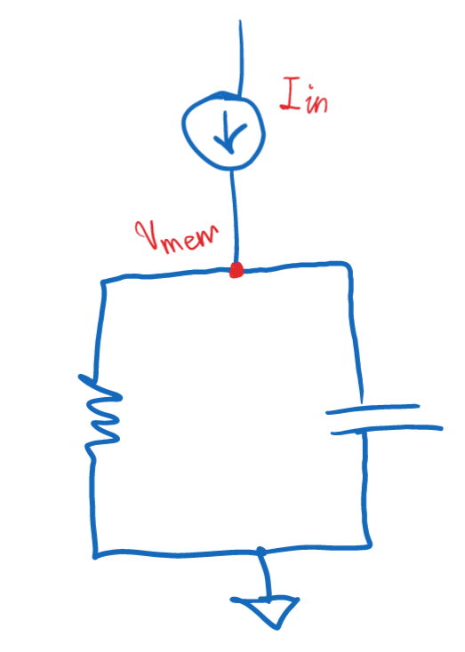
The
input current to the neuron is received as a delta Dirac function to
model spikes in the brain. The voltage of the node connecting the
resistors, the capacitor, and the input current, are called Membrane
Potential V, where it evolves according to a differential equation τ dv/dt = -V. This is referred to as leak.
When a neuron receives a spike, an increase in V is controlled by the
synaptic weight w V:= V+w, which is referred to as integrate. The last
part, fire, involves firing when the activation is above a certain
threshold called V > Vt and then resetting V := 0 afterward.
As
one dimension is barely enough to fully capture the dynamics of
neurons, a two-dimensional leaky integrate-and-fire model is used. A
dynamic threshold Vt is added, and the threshold dynamics equation is τt dVt/dt = 1 - Vt,
which decays to 1 rather than 0. After a spike, V is reset to 0 and Vt
increases by δVt. This means that Vt is constantly changing over time,
making it harder for a neuron to produce a spike while the threshold has
been increased, which leads to the next property.
Coincidence Detection
SNNs have a unique property called coincidence detection, meaning that they respond more strongly to spikes arriving at similar times super-linearly than to spikes that are spread out in time.
Input Encoding
Inputs to SNNs can be encoded in two different ways: rate codes and temporal codes. In rate codes, information is stored in the spike count or firing rate. For example, if an input has high intensity (i.e., a very bright pixel), the frequency of firing is higher. Rate codes are less error-prone and have more noise tolerance, thus more friendly with backpropagation.
On the other hand, in temporal codes, information is stored at the time of a spike. If there is a very bright pixel, the neuron will fire a very quick spike, while a dark pixel will convert to a very late spike. Timing is better for power efficiency and latency. To train a network on a rate code, each neuron’s average frequency is measured over a certain amount of time. In temporal coding, only the neuron that fires first matters.
Input encoding in Action
I will walk through a simple case for rate-coding an image using the Poisson distribution. First, let’s get an image from the CIFAR10 dataset.
batch_size_train = 64
transform_test = transforms.Compose([
    transforms.ToTensor(),
])
testset = CIFAR10('.pytorch/CIFAR10', train=False, transform=transform_test, download=True)
testloader = torch.utils.data.DataLoader(testset, batch_size=batch_size_train, shuffle=False, num_workers=2)
Then I will normalize and plot an image. The normalized pixel value represents the probability that a spike occurs for a particular pixel at any given time.
image_batch, labels_batch = next(iter(testloader))
image = image_batch[11]
# Normalizing the image
image = (image - image.min())/(image.max()-image.min())
plt.imshow(image.permute([1, 2, 0]))
plt.show()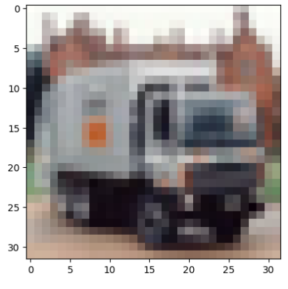
I will use 100 as the time-steps and repeat the first dimension. After repeating, I will concatenate a vector of ones with the same dimensions as images in the CIFAR10 dataset at the begging of the data.
time_steps = 100
# Repeating by the number of time_steps
raw_vector = torch.cat([
    torch.ones(1, 3, 32, 32),
    image.repeat(time_steps, 1, 1, 1)
])
It’s now time to pass the sample through the Poisson distribution.
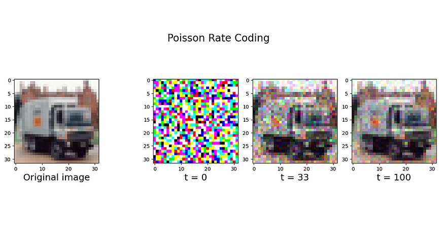
rate_coded_vector = torch.poisson(raw_vector)Finally, I plot the mean of the sample at time-steps equal to 0, 33, and 100 to see the result of the encoding.
fig, ax = plt.subplot_mosaic(
    """
    A.BCD
    """,
    figsize=(15, 5),
    gridspec_kw={'width_ratios':[1,0.3,1,1,1]}
)
fig.suptitle('Poisson Rate Coding', fontsize=20)
ax['A'].imshow(image.permute([1, 2, 0]))
ax['A'].set_xlabel('Original image', fontsize=18)
ax['B'].imshow(rate_coded_vector[0].permute([1, 2, 0]))
ax['B'].set_xlabel('t = 0', fontsize=18)
ax['C'].imshow(rate_coded_vector[:time_steps//3].mean(0).permute([1, 2, 0]))
ax['C'].set_xlabel(f't = {time_steps//3}', fontsize=18)
ax['D'].imshow(rate_coded_vector.mean(0).permute([1, 2, 0]))
ax['D'].grid(None)
ax['D'].set_xlabel(f't = {time_steps}', fontsize=18)
plt.grid(None)
plt.show()
Now as expected, as time progress toward the end, the plot converges more to the original image.
The code for this simulation and a few more hands-on examples are available on GitHub.
SNNs and Intelligence
Neurons might be the basis of the only known system for general intelligence. Yet, we don’t know how Neurons learn, though we do have observed some behaviors about how biological neurons work. Learning happens by, e.g., strengthening and weakening synapses or adding or removing synapses or neurons. Typical models of learning for neurons include reward-modulated systems, where learning is gated by some reward, and spike-timing-dependent plasticity (STDP), where the connection is strengthened if a pre-synaptic neuron fires just before a postsynaptic neuron.
Learning Methods
Spike Timing Dependent Plasticity and Online Learning
Let’s begin with STDP. This method enables neurons to adjust their synaptic weights based on the relative timing of their pre-and post-synaptic spikes. It is a form of unsupervised learning that enables lifelong learning. This method requires the model to be deployed on neuromorphic hardware and can’t be scaled beyond 2 to 3 layers of shallow networks. Thus, it cannot be extended to more complex tasks. Even if it’s used alone for feature extraction, another supervised layer must be followed for the classification layer.
To understand this method better, let’s have a look at a paper applying this approach to a digit classification task. Diehl et al. [1] used a two-layer SNN for digit classification on the MNIST dataset. First, the inputs are encoded using Poisson rate coding with exponential distribution for inter-spike intervals. In other words, if a pixel has higher intensities, it produces more spikes, and vice versa.
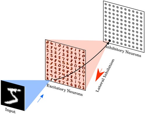
The architecture consists of an Excitatory and Inhibitory layer. Regardless of the type of layers, we have a fully connected configuration between the input and output of a layer. In the case of the excitatory layer, we let the network itself figure out the correct weight to learn some representation from the input. One caveat here, as this is fully unsupervised, neurons tend to learn greedily. Thus, spiking activity should be normalized to introduce competition among neurons to enforce learning distinct features rather than learning greedily. This means that, whenever a neuron in the excitatory layer spikes, it will inhibit all other neurons from activating by sending a signal from the inhibitory layer to the network.
Adaptive Synaptic Plasticity and Lifelong Learning
The main goal of Adaptive Synaptic Plasticity is to selectively forget unimportant information to continuously learn with constrained resources. Panda et al. leverage this to address catastrophic forgetting and enable lifelong learning.
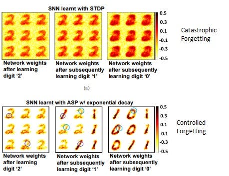
The key difference between STDP and ASP is that former weight states are only altered in case of a post-pre neuron spike, while the former leaks the weights at every time instant towards a baseline irrespective of neuron spikes [2]. In other words, updating the weight only through spike activity limits the capabilities of the layer to learn diverse representation while given frequently changing inputs.
Native Training: Learning via Backpropagation
Spiking Neural Networks, similar to Artificial Neural Networks, can be trained using backpropagation. The advantage is all the lessons we learned through 25 years of training ANNs [6] apply to SNNs in this approach. Considering the efficiency and scalability of accelerators for backpropagation, we can scale SNNs on par with ANNs. However, what is the biggest obstacle here? Spikes are modeled using the Heaviside function.
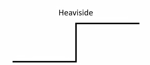
The derivative of the Heaviside function is zero for all non-zero values, thus, gradient descent can’t work.
Smooth Threshold
The first solution is to smooth out the threshold function similar to our beloved Sigmoid function to replace the Heaviside function. This means that we are compromising on fully capturing the dynamics of spikes. Plus, the decay makes the process slower. This was studied by Huh et al. [3].
Surrogate gradient descent
We only need to calculate the gradient on the backward pass. In contrast, we don’t have such a constraint on the forward pass. In work by Neftci et al. [4], this disentanglement for the two passes was used. In essence, we use Heaviside for the forward pass and a smooth threshold function like sigmoid on the backward pass. The caveat here is that we’re optimizing a different function than the function we’re evaluating on.
Shadow training: ANN-to-SNN Conversion
As stated, native training of SNNs can be very sensitive to hyperparameters. Additionally, the training process on legacy hardware is less efficient as SNNs’ intrinsic properties are not utilized in this approach. However, there is still a way to take advantage of the benefits of SNNs without having to deal with these challenges.
This technique is called shadow training, which involves converting an ANN into an SNN. By doing so, we can take advantage of SNNs while still using the efficient training methods of ANNs. Unfortunately, it doesn’t come without compromises. One of the biggest compromises is using conversion will suppress SNN to an approximation of ANN. Thus something because of this conversion is lost, leaving the network at a suboptimal point. While training, we also didn’t leverage temporal statistics of SNNs.
Neuromorphic Hardware
Ideally, neurons should be an independent, autonomous unit of computation and memory, communicating with each other. On the other hand, we have the common Von Neumann architecture, where computation is separated from memory and the I/O unit. Thus, traditional hardware is not the ideal architecture for Spiking Neural Networks. The large circuit overhead arising from having dozens of neurons makes the ideal architecture impractical [5]. To this end, a practical compromise is to group several neurons to compensate for the circuitry overhead while enjoying the benefits of close-to-memory computation. As for communication, cores are connected through routers operating only on spike events in a time-multiplexed manner [5].
Intel Loihi is the premier spiking neural network (SNN) hardware that utilizes asynchronous dynamic information processing in the form of spikes. This allows for efficient handshaking between components, ensuring that the circuit only activates when it is necessary to do so. Additionally, memory is intertwined on a fine scale with the processing elements, creating an integrated computation system.
Despite these advantages, there is a trade-off between power and accuracy to consider when using Intel Loihi hardware. Not all operations are implemented, like, e.g., maximum function for pooling operations. Furthermore, due to scalability issues, Intel Loihi hardware is not suitable for training and will require the use of a GPU instead, although it supports on-chip training.
Final Thoughts
While there is still much we don’t know about how these networks learn and operate, they are a promising area of research for both neuroscience and artificial intelligence. As we continue to develop and refine these models, we may one day unlock the secrets of the brain and create truly intelligent machines.
I will write more articles in CS. If you’re as passionate about the industry as I am ^^ and find my articles informative, be sure to hit that follow button on Medium and continue the conversation in the comments if you have any questions. Don’t hesitate to reach out to me directly on LinkedIn!
References:
[1] Diehl, Peter U., and Matthew Cook. “Unsupervised learning of digit recognition using spike-timing-dependent plasticity.” Frontiers in computational neuroscience 9 (2015): 99.
[2] Panda, Priyadarshini, et al. “Asp: Learning to forget with adaptive synaptic plasticity in spiking neural networks.” IEEE Journal on Emerging and Selected Topics in Circuits and Systems 8.1 (2017): 51–64.
[3] Huh, Dongsung, and Terrence J. Sejnowski. “Gradient descent for spiking neural networks.” Advances in neural information processing systems 31 (2018).
[4] Neftci, Emre O., Hesham Mostafa, and Friedemann Zenke. “Surrogate gradient learning in spiking neural networks: Bringing the power of gradient-based optimization to spiking neural networks.” IEEE Signal Processing Magazine 36.6 (2019): 51–63.
[5] Shrestha, Amar, et al. “A survey on neuromorphic computing: Models and hardware.” IEEE Circuits and Systems Magazine 22.2 (2022): 6–35.
[6] LeCun, Yann, et al. “Efficient backprop.” Neural networks: Tricks of the trade. Berlin, Heidelberg: Springer Berlin Heidelberg, 2002. 9–50.
https://pub.towardsai.net/the-complete-guide-to-spiking-neural-networks-d0a85fa6a64
No hay comentarios:
Publicar un comentario